How to parallelize 'do' computation in dplyr
Posted on 25 Feb 2017 RdplyrTutorial 添加评论Introduction
Recently, I took apart in the IJCAI-17 Customer Flow Forecasts. It is an interesting competition in some extent. The datasets provided include:
- shop_info: shop information data
- user_pay: users pay behavior
- user_view: users view behavior
- prediction:test set and submission format
Because the nature of this problem is to predict time series, methods specifically designed for this task should be tested. The well-known ones include:
- ARIMA series models
- ETS series models
- Regression models
And it is not hard to find out that customer flow is a seasonal time series. Therefore, time series decomposition such as X12 and STL may be useful tools in analysis.
Preprocessing
The datasets include plenty of information such as the user_id make a payment to shop_id at time. Because the goal is to predict the flow of each shop and it is hard to build a user_id profile based model with only this amount of data provided, a shop_id profile based solution appears to be a better choice, i.e., we will build a model for each shop, and do the prediction. Therefore, for the preprocessing, the user_id should be aggregated. This is a pretty entry level task for dpylr(R) or pandas(Python) user. Therefore, I do not share code for this part, the results are organized as following dataset:
library(psych)
summary(tc2017)
## shop_id time_stamp date_week nb_pay
## Min. : 1 Min. :2015-06-26 Monday :86544 Min. : 1.0
## 1st Qu.: 504 1st Qu.:2016-02-03 Tuesday :84851 1st Qu.: 51.0
## Median :1019 Median :2016-05-22 Wednesday:85283 Median : 82.0
## Mean :1008 Mean :2016-05-04 Thursday :85643 Mean : 116.3
## 3rd Qu.:1512 3rd Qu.:2016-08-15 Friday :86041 3rd Qu.: 135.0
## Max. :2000 Max. :2016-10-31 Saturday :84902 Max. :4704.0
## Sunday :86011describe(tc2017)## vars n mean sd median trimmed mad min max
## shop_id 1 599275 1007.58 577.88 1019 1008.69 747.23 1 2000
## time_stamp* 2 599275 NaN NA NA NaN NA Inf -Inf
## date_week* 3 599275 4.00 2.00 4 4.00 2.97 1 7
## nb_pay 4 599275 116.26 132.04 82 93.64 54.86 1 4704
## range skew kurtosis se
## shop_id 1999 -0.02 -1.22 0.75
## time_stamp* -Inf NA NA NA
## date_week* 6 0.00 -1.25 0.00
## nb_pay 4703 7.06 105.67 0.17Exploratory
First, let us make some figures using off course ggplot2. Plots for first five shops:
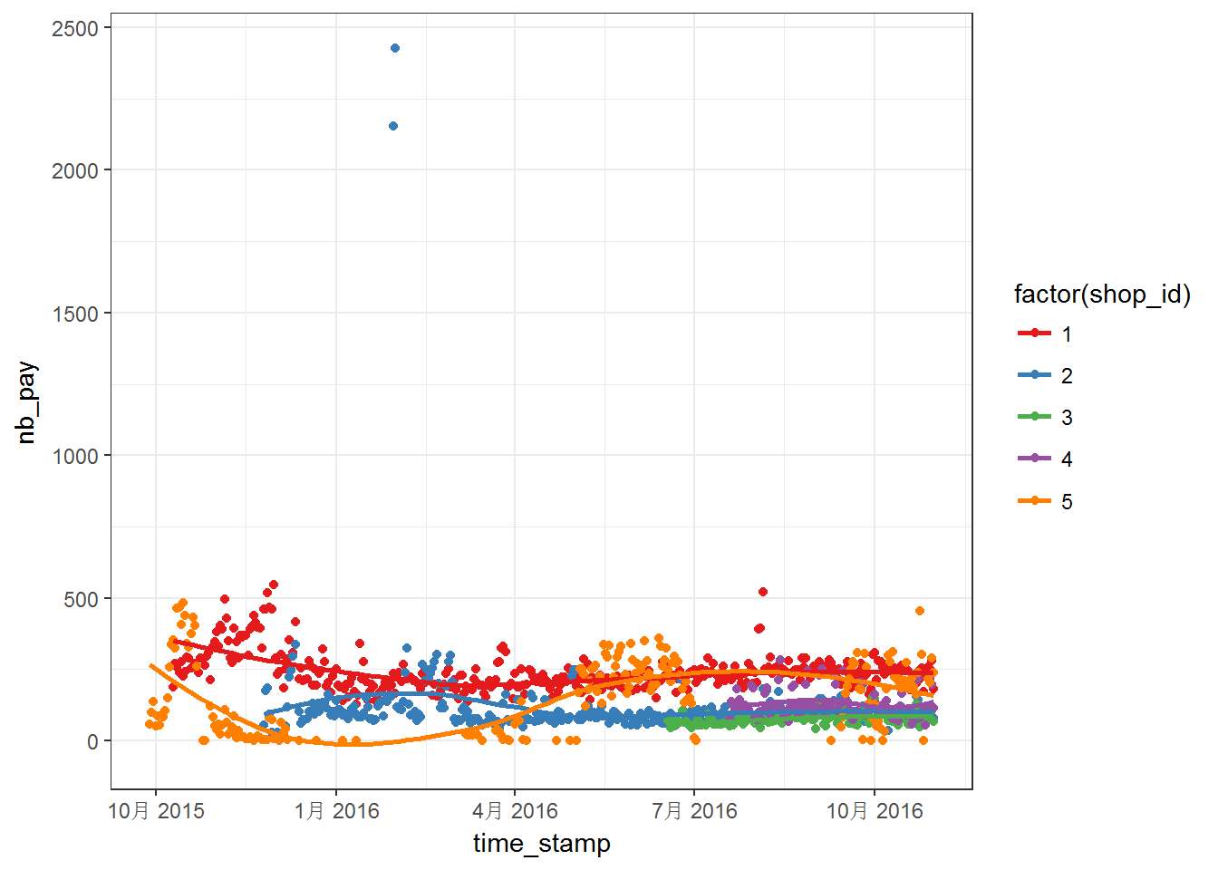
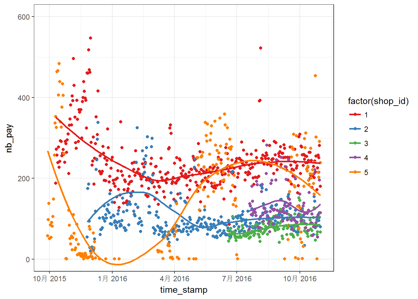
Above two figures are quite messy. We can notice that the data have different range, which means that we may have to worry about NAs. Moreover, most of the series do not steady in the given range. For these five curves, the curves are more steady after April 2016. Then, above series are plotted into separated panels as follows:
p <- ggplot(tc2017 %>% filter(shop_id<6),aes(time_stamp,nb_pay)) +
  geom_line() +
  facet_wrap(~shop_id, ncol = 1, scales = "free")
print(p)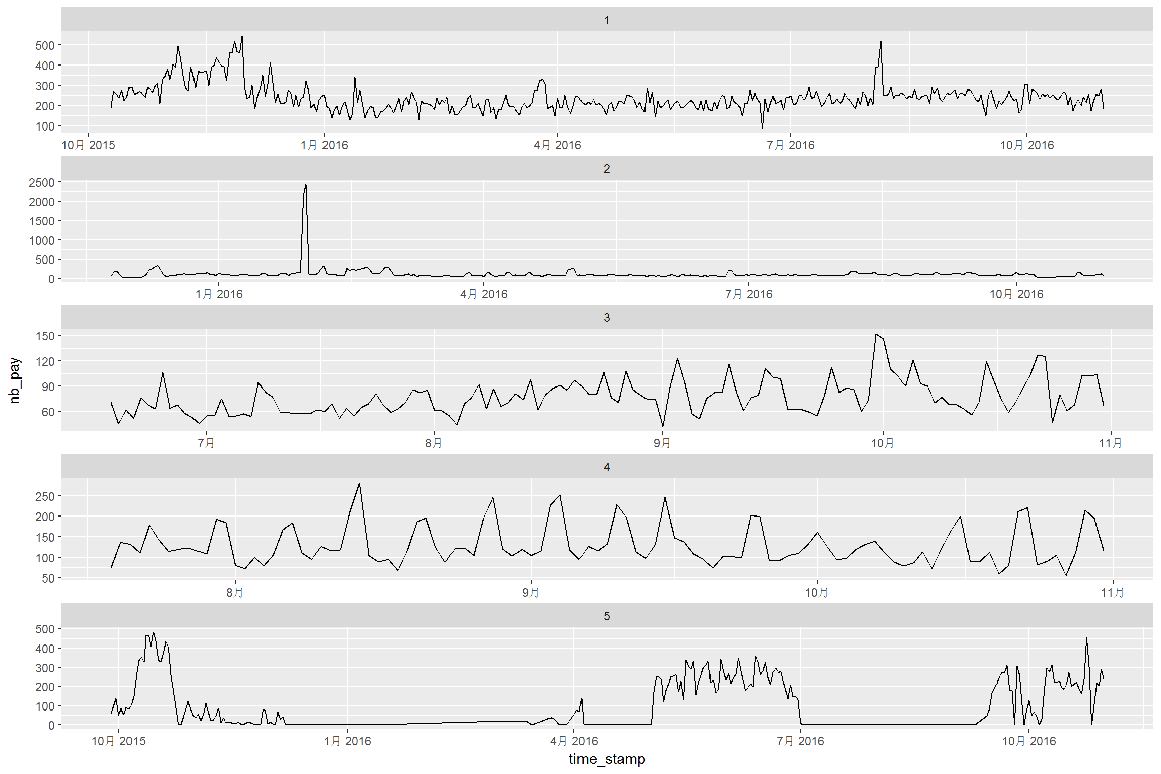
Some series have strong seasonal feature, such as curve for shop_id==4. We may need to consider the seasonal effect. A quick acf drawing is shown as below:
acf((tc2017 %>% filter(shop_id==4))$nb_pay)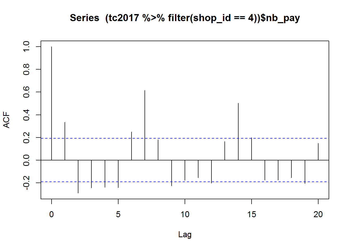
It can be observed that the periodic pattern is quite clear, the period is 7 and it is the length of one week. Therefore, we plot the data against the weekday:
p <- ggplot(tc2017 %>% filter(shop_id==4),
            aes(time_stamp,nb_pay)) +
  geom_line(size=1) +
  facet_grid(date_week~.,scales = "fixed")+
  theme_bw()
print(p)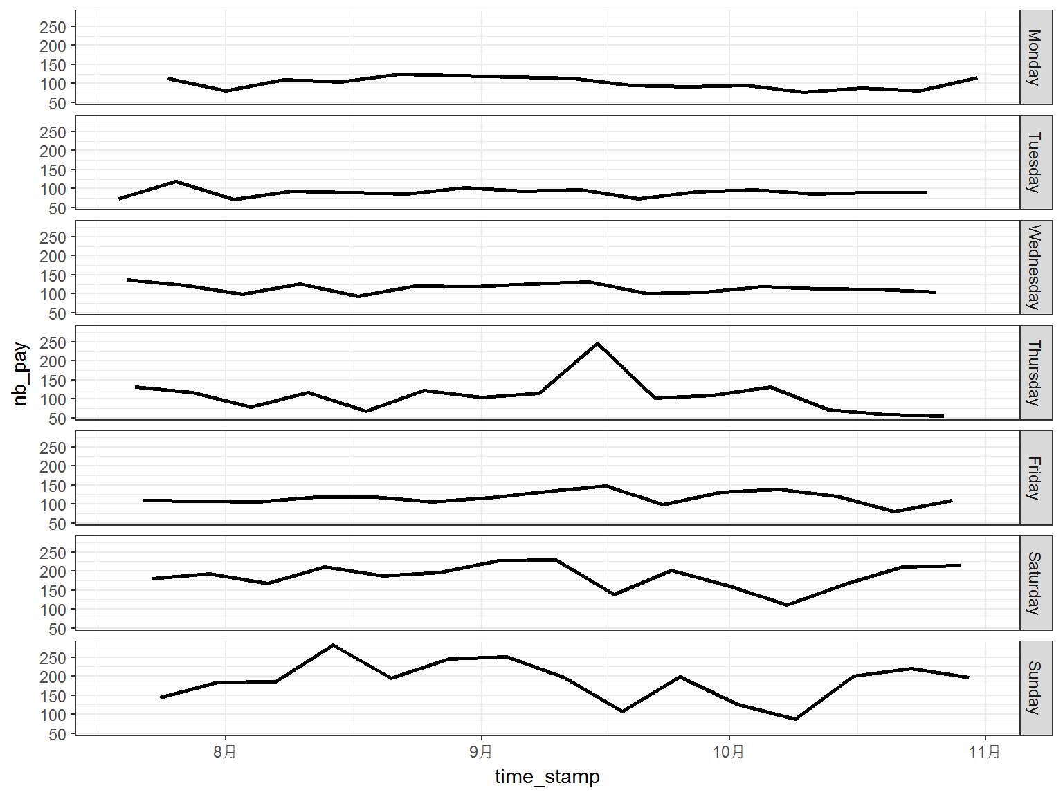
It is shown in above figure, the number of customs is much steady when we investigate the flow on the same weekday. This pattern also appears in the data of other shops.
p <- ggplot(tc2017 %>% filter(shop_id<6),
            aes(time_stamp,nb_pay,color = date_week)) +
  geom_line(size=1) +
  facet_grid(date_week~shop_id,scales = "free")+
  scale_color_brewer(palette = "Set1")+
  theme_bw()+ theme(legend.position = "none")
print(p)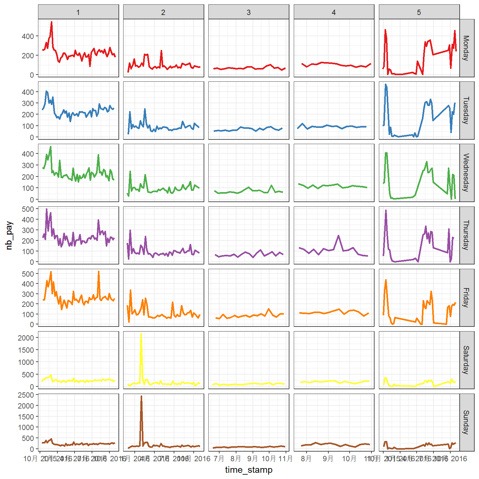
Generally, the flows have quite different patterns between weekdays and weekends. However, the longtime trend also plays important role in the flow.
Let's make some predictions here:
library(forecast)
library(xts)
to.ts <- function (x) {
  ts(x$nb_pay,frequency = 7)
}

tmp <- to.ts(tc2017%>%filter(shop_id==1))

autoplot(forecast(stlm(tmp))) + theme_bw()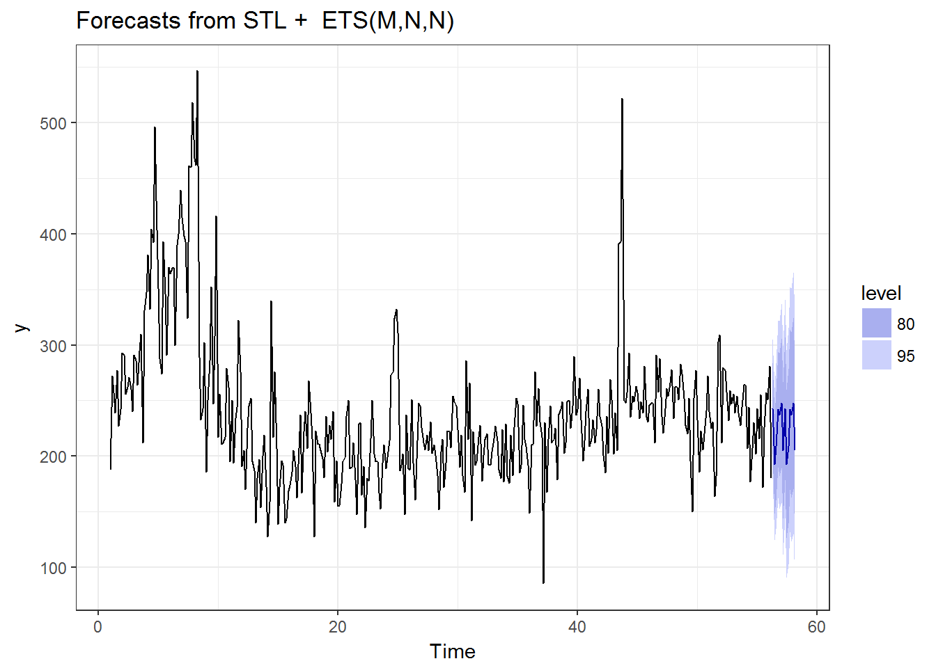
autoplot(forecast(ets(tmp))) + theme_bw()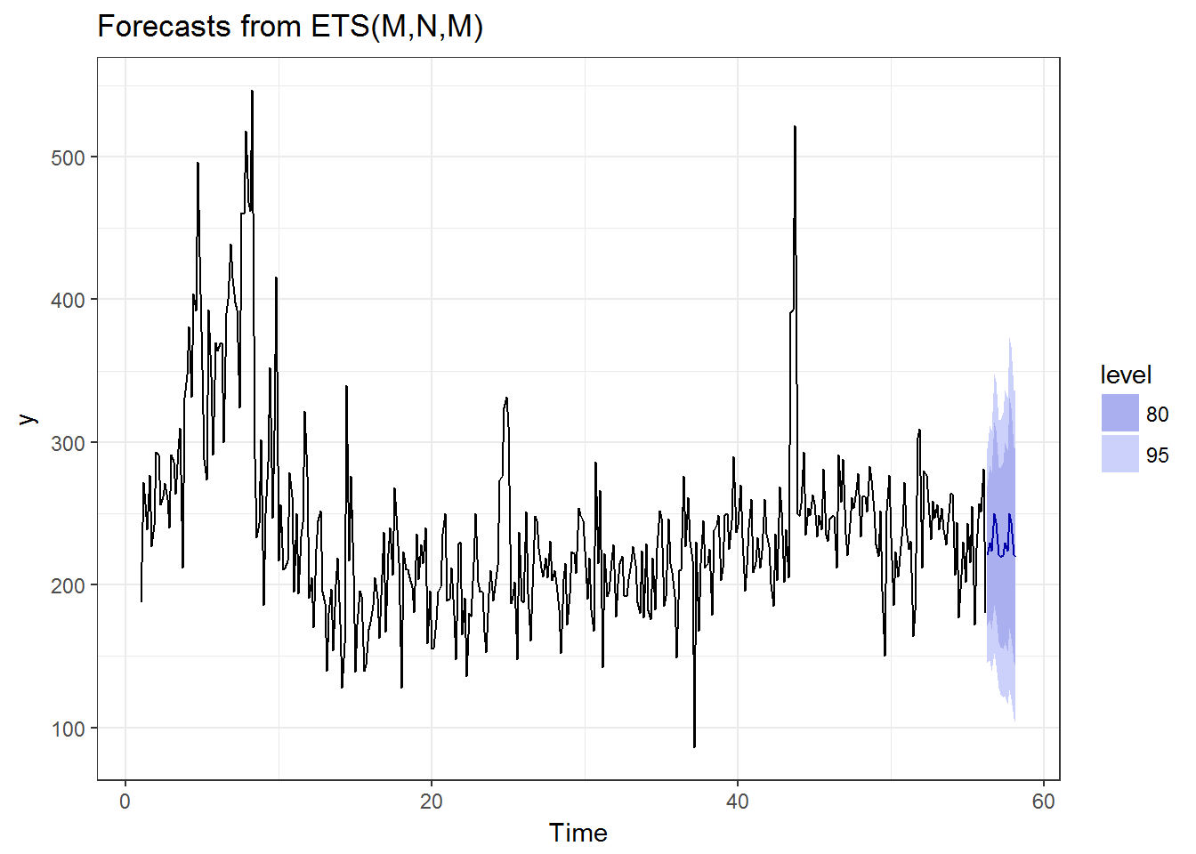
autoplot(forecast(tbats(tmp))) + theme_bw()
autoplot(forecast(auto.arima(tmp,NA,1))) + theme_bw()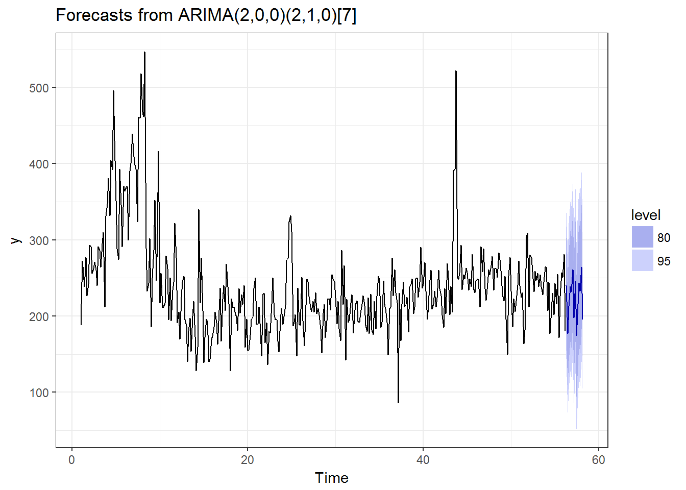 How about
 shope_id==4:
tmp <- to.ts(tc2017%>%filter(shop_id==4))

autoplot(forecast(stlm(tmp))) + theme_bw()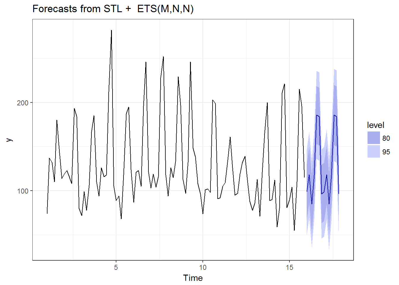
autoplot(forecast(ets(tmp))) + theme_bw()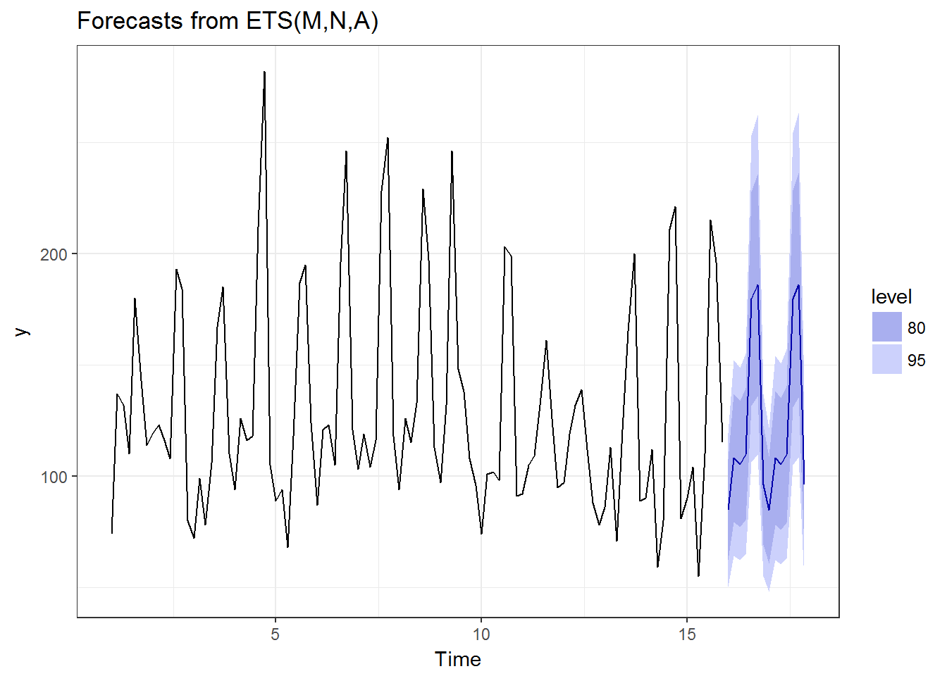
autoplot(forecast(tbats(tmp))) + theme_bw()
autoplot(forecast(auto.arima(tmp,NA,1))) + theme_bw()
OK, this is the end of the analysis, otherwise the article becomes a tutorial on analyzing the competition data. Based on the results above, the performances of the well-known methods are pretty decent in my opinion. Next is how to calculate them in 2000 shops.
A workable solution
ets is a fast algorithm, and its performance is quite good. Therefore, let's assume we want to apply ets to the whole dataset. The easiest way is to use some functions from dplyr. summarise is a good candidate, but it only able to capture functions with only one return value, such as mean and median:
tc2017 %>% group_by(shop_id) %>%
  summarise(mean(nb_pay),median(nb_pay))
## # A tibble: 2,000 × 3
## shop_id `mean(nb_pay)` `median(nb_pay)`
## <int> <dbl> <dbl>
## 1 1 239.50646 228
## 2 2 118.87538 92
## 3 3 76.97794 74
## 4 4 129.58095 116
## 5 5 155.71782 158
## 6 6 62.11765 60
## 7 7 144.79917 139
## 8 8 81.63043 76
## 9 9 182.61035 171
## 10 10 45.39024 43
## # ... with 1,990 more rowsSo, we need a general version of summarise, and what we get is do:
This is a general purpose complement to the specialised manipulation functions filter, select, mutate, summarise and arrange. You can use do to perform arbitrary computation, returning either a data frame or arbitrary objects which will be stored in a list. This is particularly useful when working with models: you can fit models per group with do and then flexibly extract components with either another do or summarise.
Here is where most people get stuck, because the first example of this function is something like:
head3## Source: local data frame [6,000 x 4]
## Groups: shop_id [2,000]
##
## shop_id time_stamp date_week nb_pay
## <int> <date> <fctr> <int>
## 1 1 2015-10-10 Saturday 188
## 2 1 2015-10-11 Sunday 272
## 3 1 2015-10-12 Monday 257
## 4 2 2015-11-25 Wednesday 55
## 5 2 2015-11-26 Thursday 175
## 6 2 2015-11-27 Friday 186
## 7 3 2016-06-18 Saturday 71
## 8 3 2016-06-19 Sunday 45
## 9 3 2016-06-20 Monday 62
## 10 4 2016-07-19 Tuesday 74
## # ... with 5,990 more rowsAbove function extracted the first three values appearing for each shop. The data structure what we get is the same as the original one. Pretty good? No, what we need is You can use do to perform arbitrary computation, returning either a data frame or arbitrary objects which will be stored in a list. And the first example absolutely sent us to a wrong direction. Actually, the later examples did the right thing. The trick is to assign the return value to a variable:
head3## Source: local data frame [2,000 x 2]
## Groups: <by row>
##
## # A tibble: 2,000 × 2
## shop_id head3
## * <int> <list>
## 1 1 <int [3]>
## 2 2 <int [3]>
## 3 3 <int [3]>
## 4 4 <int [3]>
## 5 5 <int [3]>
## 6 6 <int [3]>
## 7 7 <int [3]>
## 8 8 <int [3]>
## 9 9 <int [3]>
## 10 10 <int [3]>
## # ... with 1,990 more rowsAnd the head3 column is what we want:
head3$head3[1]## [[1]]
## [1] 188 272 257OK, good. The next thing is to write a forecast function and apply it the dataset. forecast library is what we are looking for.
library(forecast)
forecast.by.ets <- function(df){
  forecast(ets(to.ts(df)),14)$mean
}
Let's test this function:
forecast.by.ets(tc2017%>%filter(shop_id==1))## Time Series:
## Start = c(56, 3)
## End = c(58, 2)
## Frequency = 7
## [1] 220.4800 229.6598 223.8705 250.1321 243.6516 221.6542 219.3051
## [8] 220.4803 229.6601 223.8707 250.1323 243.6519 221.6545 219.3053OK, it seems working. Then applying it to the whole dataset:
out <- tc2017 %>% group_by(shop_id) %>%
do(predict = forecast.by.ets(.))Above function is correct. Why I leave it there is that it is so slow for our goal and here comes what this article about: how to parallelized this computation? But first let me show you above function do works:
out <- tc2017 %>% filter(shop_id<3) %>%
group_by(shop_id) %>%
do(predict = forecast.by.ets(.))
out## Source: local data frame [2 x 2]
## Groups: <by row>
##
## # A tibble: 2 × 2
## shop_id predict
## * <int> <list>
## 1 1 <S3: ts>
## 2 2 <S3: ts>out$predict[1]## [[1]]
## Time Series:
## Start = c(56, 3)
## End = c(58, 2)
## Frequency = 7
##  [1] 220.4800 229.6598 223.8705 250.1321 243.6516 221.6542 219.3051
## [8] 220.4803 229.6601 223.8707 250.1323 243.6519 221.6545 219.3053Parallelize it
Finally, all the stuffs that we need are prepared. Now the problem is following code only run in one core, which is a total waste. Come on, these jobs are perfectly separated from each other.
out <- tc2017 %>% group_by(shop_id) %>%
do(predict = forecast.by.ets(.))Yes, you can just ignore dplyr function and write your own parallel version using something like foreach or parallel. However, luckily there is a simple solution for this problem by the author of ggplot2. He provided a very elegant way to solve this problem. The library is named multidplyr. (NOT multiplyr)
library(multidplyr)multidplyr is a fantastic library. The best thing about multidplyr is that you need very little modification of your original dplyr version codes, and multidplyr will take care of almost all the other things. For our case, the codes become:
out <- tc2017 %>% partition(shop_id) %>%
  do(predict = forecast.by.ets(.)) %>%
  collect()
What is the difference? The group_by function is changed to partition, and we need to collect the data to its original format using collect. So basically, you need nothing to do, right? Clearly above code can not run correctly. At least, we need some kind of broadcast even we do not need sync in this case. In order solve this you will need some codes like:
cluster <- get_default_cluster()
cluster_library(cluster, "forecast")
cluster_library(cluster, "dplyr")

cluster_assign_value(cluster,"forecast.by.ets",forecast.by.ets)
cluster_assign_value(cluster,"to.ts",to.ts)
You may need to change some codes above for your own prediction function. Basically, you will need all the libraries and functions are correctly loaded in all the cluster nodes. Because our jobs are perfectly separated from each other, there is no need for sync data between nodes which is much easier for us and also faster.
To conclude, parallelize dplyr do function is easy by using multidplyr. Normally you need a dplyr version working code first. Because we are more familiar with it, and it is much easier to debug the dplyr version code than the parallelized version. After you have working dplyr version solution, you can use multidplyr to partition the problem and distribute them to a cluster. This is a well-designed framework, although it cannot dealing with more serious parallelize problem requiring communication between nodes.
BTW, multidplyr is not available in CRAN, the multiplyr in CRAN is not what we are looking for. You need devtools to install multidplyr (if you do not have devtools, install it with the commented line below.):
# install.packages("devtools")
devtools::install_github("hadley/multidplyr")